Although I’ve worked with machine learning for over six years—mostly in variational inference, energy-based models, and normalizing flows — I had never implemented a generative adversarial network (or GAN) from scratch until recently. My antagonism towards GANs stemmed from (possibly outdated) misunderstandings — many of which were perpetuated due to a variety of different interpretations from many different papers, blogposts and articles.

However, curiosity piqued my interest after reading up on implicit density ratio estimation, noise contrastive estimation and their uses in implicit variational inference among other things; so I knew I had to give GANs a shot.

Rather than following existing tutorials, I approached the task the way I’ve always understood generative modeling: through the lens of divergence minimization and density ratio estimation.

The Perspective: Ratio Estimation Meets Divergence Minimization

This framing comes directly from two pivotal papers:

• Improved Generator Objectives for GANs — Poole et al., 2016
• f-GAN: Training Generative Neural Samplers using Variational Divergence Minimization — Nowozin, Cseke, and Tomioka, 2016

They recast GAN training as a two-step process:

1. Train the discriminator to estimate the log-density ratio between data and generator distributions.
2. Train the generator to minimize a divergence to the data distribution, using the discriminator’s output.

Instead of treating GANs as black-box adversarial games, this gives us a principled statistical foundation that feels at home in the world of variational methods and EBMs.

The Discriminator: Log-Ratio Estimation via BCE

In my implementation, the discriminator outputs raw logits (no sigmoid activation function), and is trained using binary cross-entropy with logits:

disc_real_loss = F.binary_cross_entropy_with_logits(disc(x_real), disc_real, reduction='mean')
disc_fake_loss = F.binary_cross_entropy_with_logits(disc(x_fake.detach()), disc_fake, reduction='mean')
disc_loss = disc_real_loss + disc_fake_loss

This is not just a convenient trick — it’s essential. Under this loss, the discriminator \(D_\phi(x)\) approximates:

That is, the log-density ratio between real and generated data. The density ratio appears in the optimal discriminator in standard GAN theory, and is a key ingredient in many f-divergences. Estimating it directly enables flexible generator objectives rooted in statistical inference. This subtle detail — using logits directly — turns the discriminator from a classifier into a density ratio estimator, making it a meaningful statistical object.

The Generator: Divergence Minimization with Control

Once the discriminator estimates the log-ratio, the generator can minimize a divergence of your choice — still using samples from the generator itself.

Reverse KL

This is the most straightforward loss, which can be implemented as:

log_ratio = disc(x_fake).squeeze()
gen_loss = -log_ratio.mean()

This corresponds to minimizing the reverse KL divergence \(D_{KL}(p_g(x)||p_{data}(x)) = \mathop{\mathbb{E}}_{p_g(x)}[\ln \left( \frac{p_g(x)}{p_{data}(x)} \right)]\)

This objective is mode-seeking, which is a property that often leads to sharp samples. But in practice, it doesn’t necessarily suffer from mode collapse due to the entropy regularization term in the objective, which allows the generator to generate sufficiently diverse samples.

Rényi \(\alpha\)-Divergence

Reverse KL — which is mode seeking — is a limiting case of the Rényi \(\alpha\)-divergence when \(\alpha -> 1\). The divergence takes the following form:

Letting \(\alpha → 0\) recovers an even more mode seeking objective, while increasing the value of \(\alpha\) makes the divergence more mode covering. In code, the \(\alpha\)-divergence takes the form:

alpha = 0.001 # abritrarily close to 0
gen_loss = (1 / (alpha - 1)) * (
    torch.logsumexp((1 - alpha) * log_ratio, dim=0) - math.log(batch_size)
)

The above implementation is a numerically stable equivalent of the expectation, letting us minimize a good enough estimate of the divergence using samples from the generator.

Forward KL

Interestingly, we do also have the option to minimize the forward KL divergence, despite being an expectation under the true data density rather than the model density as is the case for the GAN objective. To do so, we need to reweight the log density ratio estimate as output by the discriminator by \(\frac{p_{data}(x)}{p_g(x)}\) (i.e. the exponential of the discriminator output), which changes the density under which the expectation is taken. The forward KL is particularly interesting since it is equivalent to maxmium likleihood, which is the objective for density estimators like variational autoencoders. Thus, a GAN trained with forward KL can also be thought of as maximizing likleihood of data. Unfortunately, training with forward KL tends to collapse on random noise, which I suppose is the optimal solution as far as maximum likelihood estimation is concerned; especially since the generator has a degenerate structure. The reverse KL divergence and mode seeking \(\alpha\)-divergences give the best results, at least as far as the network parameterization goes.

Results and Reflections

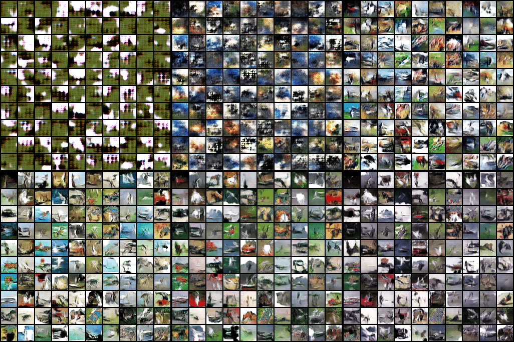
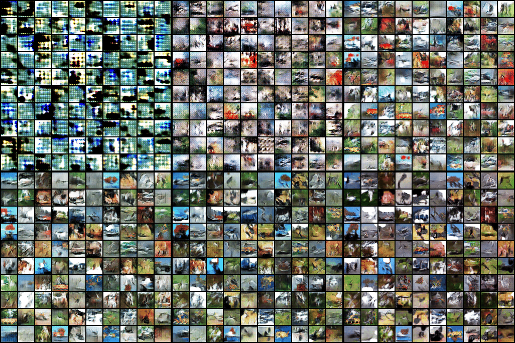
Here are the evolution of generator samples over the course of 100 iterations. The models were trained on the CIFAR-10 dataset using the same architecture and hyperparameters for each:

Both losses — reverse KL and Rényi \(\alpha → 0\) — gave me:

• Stable training
• Sharp and diverse samples
• No noticeable mode collapse (even under reverse KL)

Just by looking at the samples, it seems that the presence of entropy in reverse KL doesn’t really encourage greater sample diversity compared to the \(\alpha → 0\) divergence, although a proper log likelihood estimate would be needed in order to quantify this — perhaps by training both generators with normalizing flows.

What stood out most was the clarity and stability this perspective gave me. I wasn’t playing with any heuristics, but optimizing well-defined divergences with known statistical meaning.

Final Thoughts

This first GAN project was deeply satisfying — not because it broke new ground technically, but because it was grounded in the principles I care about: inference, optimization, and expressive modeling.

Key takeaways:

• GANs can be trained using statistically meaningful divergences, not just heuristic losses.
• The discriminator should be interpreted as a density ratio estimator, not just a classifier.
• Approximating forward KL with density ratio rescaling divergence lets you retain a generator-side expectation (though I wouldn’t recommend it!).
• Mode seeking divergences can be stable and performant; provided it is a proper divergence.

Importantly, by reframing GAN training through this statistical lens, not only can I reason about this class of models with clarity, but the implementation is actually a lot simpler and (at least in my experiments) more stable. GANs, when framed this way, feel less like unstable black-box tools and more like variational inference algorithms in disguise.

Extra notes

Wasserstein GANs (Arjovsky, Chintala and Bottou, 2016) have very little in common with ‘vanilla’ GANs; unlike the min-max optimization scheme that minimizes the Jensen-Shannon divergence, WGANs minimize the Wasserstein distance, which results in a scheme that resembles variational energy based modeling (Grathwohl et al. 2021), where the generator is matched to the discriminator / energy function to generate approximate samples from the latter; then, the discriminator / energy model penalizes those approximate samples in the standard contrastive divergence training scheme. The generator objective for the variational EBM is the reverse KL divergence, which notably imposes entropy regularization to prevent mode collapse (and results in a good density model). In WGANs, there is no such entropy regularization, which could suggest why there’s a whole host of other issues pertaining WGAN training.

References

1. Mohamed, S., & Lakshminarayanan, B. (2017). Learning in Implicit Generative Models. arXiv:1610.03483
2. Gutmann, M., & Hyvärinen, A. (2010). Noise-contrastive estimation: A new estimation principle for unnormalized statistical models. In Proceedings of the Thirteenth International Conference on Artificial Intelligence and Statistics (AISTATS), PMLR, Vol. 9, pp. 297–304. Link
3. Makhzani, A. (2019). Implicit Autoencoders. arXiv:1805.09804
4. Mescheder, L., Nowozin, S., & Geiger, A. (2018). Adversarial Variational Bayes: Unifying Variational Autoencoders and Generative Adversarial Networks. arXiv:1701.04722
5. Poole, B., Ozair, S., van den Oord, A., Alemi, A. A., & Tucker, G. (2016). Improved generator objectives for GANs. arXiv:1612.02780
6. Nowozin, S., Cseke, B., & Tomioka, R. (2016). f-GAN: Training Generative Neural Samplers using Variational Divergence Minimization. arXiv:1606.00709
7. Arjovsky, M., Chintala, S., & Bottou, L. (2017). Wasserstein GAN. arXiv:1701.07875
8. Grathwohl, W., Kelly, J., Hashemi, M., Norouzi, M., Swersky, K., & Duvenaud, D. (2021). No MCMC for me: Amortized sampling for fast and stable training of energy-based models. arXiv:2010.04230