Neural networks are all the rage in nowadays. These brain-inspired architecture that power many of todays applications are capable of recognizing images and playing video games at superhuman levels, as well as generate art and perform robotics tasks.

But are they really that intelligent? At the heart of neural networks, all that’s happening is multi-layer, multidimensional regression (or classification). Under this assumption, there are a lot of downsides that come with using NNs. These include: high data and compute requirements, having to fine-tune models to operate in a stable manner, and lack of generalization. In contrast, a human child can recognize an object in a variety of scenarios after having seen as little as one example, all while using enough electricity to power a single lightbulb.

So, is there a machine learning model that is capable of generalizing in the same way as the human brain does? The AI and robotics lab Vicarious developed a model called the Recursive Cortical Network, which proved to break CAPTCHAs in a very data-efficient manner. The point however is not to break CAPTCHAs, but rather to highlight how the design choices of this model has given it common-sense-like properties.

For those who are into neuroscience (like me :) ), you may assume that this new architecture is modelled after the neocortex (more specifically, the primary visual cortex). For those who come from a deep learning background however (I am also assuming that you have a solid background in generative modelling), this model may seem quite vague, which is why I will be explaining how this model works from a machine learning and Bayesian perspective.

What the heck is a Recursive Cortical Network?

Before moving on further, you should know that the RCN is not a neural network (in the sense that it is not performing matrix-multiplication), but a probabilistic graphical model. This means that it constructs a data generating model (or a generative model) that specifies how an image is generated from a set of latent variables. This generative model can be used to sample data similar to data it is modelling, or can be used to infer latent variables (“inference by generation”).

RCN is a lot more neurally-grounded than neural networks, separating objects from the background, and texture of an object from its shape.

Why not just use a GAN or a VAE?

One slight nitpick: Generative Adversarial Networks (GANs) and variational autoencoders (VAEs) are not actually neural networks. Rather, they are a framework for training generative models that are parameterized by some differentiable function, which may or may not be a neural network (if you do not believe me, try training a simple linear model using the mix-max game).

Traditionally, deep generative models assume that the data has been holistically generated from noise that is sampled from a probability distribution. While this is good for density estimation, this assumption is not rich enough for the sort of tasks that the RCN is naturally able to handle.

Some deep generative models like VAEs come with an inference network as a byproduct of training, which can perform fast bottom up inference of the posterior distribution. However, under the Stochastic Gradient Variational Bayes framework, only a single query can be solved through the training scheme. When another observed variable is used for querying, another network are required, which is unfeasable to train in practice. Unlike VAEs, RCN is able to perform classification, segmentation, imputation and generation all in the same model using loopy belief-propagation.

Learning an RCN

When learning an RCN, we are learning model of the shape of the image (the contours). As such, we want to be able to generate the shape of the object from this model.

Preprocessing

In order to learn an RCN, the training image must be passed through an edge detector to separate the edges. However, we can’t simply run any edge detector like the Canny edge detector, since it will not contain useful information of the features of the image. Instead, a set of Gabor filters are used, which are oriented filters that activate under the presence of a specfic edge at a specfic orientation. Neuroscience-enthusiasts may recognize this as performing the same function as simple cells. Usually, the number of filters is set to 16 (there are 16 oriented edge filters), although it can be set to a higher number for more intricacy. When the image is passed through the filters, the output should result in an array in the form of (num_filters, width, height), with each (width, height) element of the array containing edges of that particular edge-orientation. When the entire array is flattened, it results in an edge-map corresponding to the contours of the image:

Sparsification

Unlike neural networks, RCNs do not learn through backpropagation. Instead, they learn using dictionary learning. This dictionary learning algorithm greedily sparsifies the edge-map by detecting edge activations and suppressing all other activations within a certain radius. The edge activations that are detected are then stored in a dictionary in the form of (f, r, c) tuples, with correspond to the feature index (edge orientation), row and column of the activated edge respectively. This dictionary makes up the latent variables of the RCN model, unlike randomly sampled noise that VAEs and GANs assume in their data-generating procedure. To better understand the algorithm, here is some code from the reference implementation (which I slightly modified due to bugs) that highlights it into more detail:

def sparsify(bu_msg, suppress_radius=3):
    """
    Make a sparse representation of the edges by greedily selecting features from the
    output of preprocessing layer and suppressing overlapping activations.

    Parameters
    ----------
    bu_msg : 3D numpy.ndarray of float
        The bottom-up messages from the preprocessing layer.
        Shape is (num_feats, rows, cols)
    suppress_radius : int
        How many pixels in each direction we assume this filter
        explains when included in the sparsification.

    Returns
    -------
    frcs : see train_image.
    """

    frcs = []
    img = bu_msg.max(0) > 0
    for (r, c), _ in np.ndenumerate(img):
        if img[r, c]:
            frcs.append((bu_msg[:, r, c].argmax(), r, c))
            img[r - suppress_radius:r + suppress_radius + 1, 
                c - suppress_radius:c + suppress_radius + 1] = False
    return np.array(frcs)

When visualized, it results in a sparser edge map:

That is all that is needed for learning the latent variables. The next step is to construct the graphical model itself.

Lateral learning

Lateral connections play a big role in how the visual-cortex operates. And naturally, it is also present in the RCN model as well. The bare minimum for learning the RCN techically ends at the sparse dictionary learning stage, but it is shown that connections between these features improve inference in the model.

Once the latent variables have been learned through dictionary learning, the next step is to construct a graph that constrains the model. This is needed since the graph themselves do not add any randomness to the model, and thus any images sampled from the model won’t have any variation. This randomness is acheived through something called a pooling layer, which stochastically shifts the activated features inside a certain radius. However, without any constrainment, the resulting image may have too much variation and not resemble the image that it is to model. Lateral connections prevent that from happening.

Learning lateral connections are constructed done by greedily adding pairwise edges between the features, starting from the closest to the longest. The resulting graph contains connections both short and long, and it should resemble the image that is being modelled:

Once the graph is learned, the learning step is complete. Now we can move on to the inference stage.

Inference in the RCN

When performing inference, we are not just limited to classification. We can also perform generation (as it is a generative model), as well as segmentation through top down attention (which is acheived through explaining away and lateral connections). This makes it suitable for use in applications that require a flexible vision system, such as robotics. Inference in this model is a two step procedure, requiring both forward and backward passes.

Forward pass

RCNs perform Bayesian inference, which is time and computation expensive. On loopy graphs, this is even harder since finding the exact marginal is impossible, and requires approximations to be made instead. Thankfully, message passing belief propagation allows for forward passes, and a good enough approximation can be found by using some neat tricks.

In the forward pass, the input image is first passed through the Gabor filters. Afterwards, a graph cut is performed to turn the loopy graph into a tree. This allows for exact inference to be performed quite quickly through all of the graphs using the max-product algorithm. For general purpose use, this forward pass is all that is needed, but it has the tendencey to over-estimate the marginals and produce wrong assumptions. Therefore, the forward pass is used to select a set of candidate hypothesis (a group of high scoring graphs) that will be explained away in the backward pass.

Backward pass

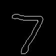
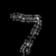
In the backward pass, the cadidates that were selected in the forward pass will be refined through loopy belief propagation on the full graph. This time around, multiple iterations of loopy belief propagation is performed to explain away any conflicting variables. When the inference is complete, the backtraced latent variables (in the form of (f, r, c)) are decoded into the edge map, resulting in top down attention. It is at this stage that the RCN can explain away noisy and occluded images, such as the example below with an occluded “7”:

Occluded image

Backtrace

And that is inference in the RCN!

That sounds cool! Why aren’t we using it in practice?

Long story short, RCNs also have drawbacks, some of which that deep learning does not have to deal with. As a probabilistic graphical model, a lot of prior knowledge is incorporated into this architecture, leading to design choices that do not necessarily work in the real world. At the moment, RCN only models shape; texture and colour have to be modelled separately using a conditional random field, for which bottom up inference is not yet available. Furthermore, RCNs require clean data samples, which is not readily available in the real world (neural networks bypass this by learning the average features of their training data). The pooling in the RCN also has some drawbacks in that it constraining it too much leads it to failing to recognize certain objects (for example, it is not able to recognize a chair that looks different from the one it has been trained on), and making it too flexible leads it to making wrong assumptions. Nonetheless, the work in this paper is a small step in making artificial intelligence models that can learn and generalize in the same way as humans.

Acknowledgements

The images in this post were possible with the help of the research paper, the supplementary paper, and the reference implementation of the RCN.

Code for visualizations

The code that I used to visualize the RCN model is located here